Binary Indexed Trees - Algorithm Tutorials

https://www.hackerearth.com/practice/data-structures/advanced-data-structures/fenwick-binary-indexed-trees/tutorial/

Using binary Indexed tree also, we can perform both the tasks in O(logN) time. But then why to learn another data structure when segment tree can do the work for us. It’s because binary indexed trees require less space and are very easy to implement during programming contests (the total code is not more than 8-10 lines).

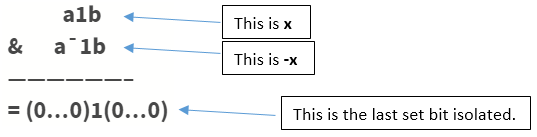
x & (-x) gives the last set bit in a number $x$. How?

Say $x=a1b$(in binary) is the number whose last set bit we want to isolate.

Here $a$ is some binary sequence of any length of 1’s and 0’s and $b$ is some sequence of any length but of 0’s only. Remember we said we want the LAST set bit, so for that tiny intermediate 1 bit sitting between a and b to be the last set bit, b should be a sequence of 0’s only of length zero or more.

-x = 2’s complement of x = (a1b)’ + 1 = a’0b’ + 1 = a’0(0….0)’ + 1 = a’0(1...1) + 1 = a’1(0…0) = a’1b

Example: x = 10(in decimal) = 1010(in binary)

The last set bit is given by x&(-x) = (10)1(0) & (01)1(0) = 0010 = 2 (in decimal)

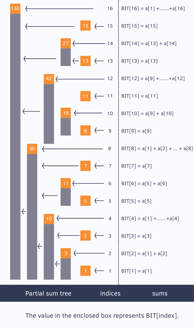
We know the fact that each integer can be represented as the sum of powers of two. Similarly, for a given array of size $N$, we can maintain an array $BIT[]$ such that, at any index we can store the sum of some numbers of the given array. This can also be called a partial sum tree.

Let’s use an example to understand how $BIT[]$ stores partial sums.

//for ease, we make sure our given array is 1-based indexed
int a[] = {0, 1, 2, 3, 4, 5, 6, 7, 8, 9, 10, 11, 12, 13, 14, 15, 16};

The above picture shows the binary indexed tree, each enclosed box of which denotes the value $BIT[index]$ and each $BIT[index]$ stores partial sum of some numbers.

Notice

               {           a[x],                  if x is odd
BIT[x] =                    a[1] + ... + a[x],     if x is power of 2
               }

To generalize this every index $i$ in the $BIT[]$ array stores the cumulative sum from the index $i$ to $i-(1<<r)+1$ (both inclusive), where $r$represents the last set bit in the index $i$.

Sum of first 12 numbers in array $a[]=BIT[12]+BIT[8]=(a[12]+\dots +a[9])+(a[8]+\dots +a[1])$

Similarly, sum of first 6 elements $=BIT[6]+BIT[4]=(a[6]+a[5])+(a[4]+\dots +a[1])$

Sum of first 8 elements$=BIT[8]=a[8]+\dots +a[1]$

Let’s see how to construct this tree and then we will come back to querying the tree for prefix sums. $BIT[]$ is an array of size = 1 + the size of the given array $a[]$ on which we need to perform operations. Initially all values in $BIT[]$ are equal to $0$. Then we call update() operation for each element of given array to construct the Binary Indexed Tree. The update() operation is discussed below.

void update(int x, int val)       //add "val" at index "x"
{
    for(; x <= n; x += x&-x)
          BIT[x] += val;
}




Suppose we call update(13, 2).

Here we see from the above figure that indices 13, 14, 16 cover index 13 and thus we need to add 2 to them also.

Initially $x$ is 13, we update $BIT[13]$

    BIT[13] += 2;

Now isolate the last set bit of $x=13(1101)$ and add that to $x$ , i.e. x += x&(-x)$\text{x += x\&(-x)}$

Last bit is of $x=13(1101)$ is $1$ which we add to $x$, then $x=13+1=14$, we update $BIT[14]$

    BIT[14] += 2;

Now $14$ is $1110$, isolate last bit and add to $14$, $x$ becomes $14+2=16(10000)$, we update $BIT[16]$

    BIT[16] += 2;

In this way, when an update() operation is performed on index $x$ we update all the indices of $BIT[]$ which cover index $x$ and maintain the $BIT[]$.

If we look at the for loop in update() operation, we can see that the loop runs at most the number of bits in index $x$ which is restricted to be less or equal to $N$ (the size of the given array), so we can say that the update operation takes at most $O(logN)$ time.

How to query such structure for prefix sums? Let’s look at the query operation.

int query(int x)      //returns the sum of first x elements in given array a[]
{
     int sum = 0;
     for(; x > 0; x -= x&-x)
         sum += BIT[x];
     return sum;
}

The above function query() returns the sum of first $x$ elements in given array. Let’s see how it works.

Suppose we call query(14), initially sum = 0
$x$ is $14(1110)$ we add $BIT[14]$ to our sum variable, thus $sum=BIT[14]=(a[14]+a[13])$

Now we isolate the last set bit from $x=14(1110)$ and subtract it from $x$
Last set bit in $14(1110)is2(10)$, thus $x=14–2=12$

We add $BIT[12]$ to our sum variable, thus $sum=BIT[14]+BIT[12]=(a[14]+a[13])+(a[12]+\dots +a[9])$

Again we isolate last set bit from $x=12(1100)$ and subtract it from $x$
Last set bit in $12(1100)$ is $4(100)$, thus $x=12–4=8$

We add $BIT[8]$ to our sum variable, thus

$sum=BIT[14]+BIT[2]+BIT[8]=(a[14]+a[13])+(a[12]+\dots +a[9])+(a[8]+\dots +a[1])$

Once again we isolate last set bit from $x=8(1000)$ and subtract it from $x$
Last set bit in $8(1000)$ is $8(1000)$, thus $x=8–8=0$

Since $x=0$, the for loop breaks and we return the prefix sum.

Talking about time complexity, again we can see that the loop iterates at most the number of bits in $x$ which will be at most $N$ (the size of the given array). Thus, the *query operation takes $O(logN)$ time 

Before going for Binary Indexed tree to perform operations over range, one must confirm that the operation or the function is:

Associative. i.e $f(f(a,b),c)=f(a,f(b,c))$ this is true even for seg-tree

Has an inverse. eg:

1. Addition has inverse subtraction (this example we have discussed)
2. Multiplication has inverse division
3. $gcd()$ has no inverse, so we can’t use BIT to calculate range gcd’s
4. Sum of matrices has inverse
5. Product of matrices would have inverse if it is given that matrices are degenerate i.e. determinant of any matrix is not equal to 0

Space Complexity: $O(N)$ for declaring another array of size $N$

Time Complexity: $O(logN)$ for each operation(update and query as well)

Applications:

1. Binary Indexed trees are used to implement the arithmetic coding algorithm. Development of operations it supports were primarily motivated by use in that case.
2. Binary Indexed Tree can be used to count inversions in an array in $O(NlogN)$ time.

https://www.geeksforgeeks.org/binary-indexed-tree-or-fenwick-tree-2/

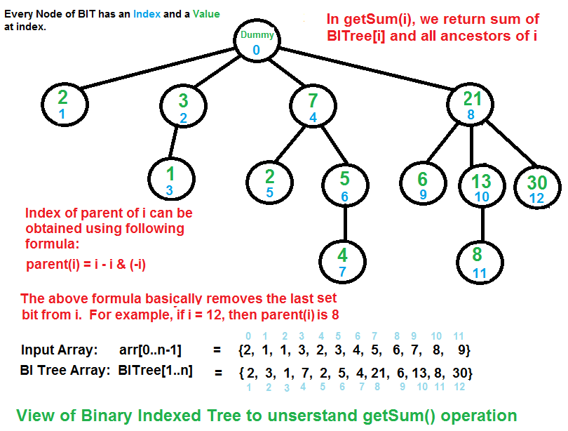
getSum(x): Returns the sum of the sub-array arr[0,...,x]
// Returns the sum of the sub-array arr[0,...,x] using BITree[0..n], which is constructed from arr[0..n-1]
1) Initialize the output sum as 0, the current index as x+1.
2) Do following while the current index is greater than 0.
...a) Add BITree[index] to sum
...b) Go to the parent of BITree[index].  The parent can be obtained by removing
     the last set bit from the current index, i.e., index = index - (index & (-index))
3) Return sum.

The diagram above provides an example of how getSum() is working. Here are some important observations.

BITree[0] is a dummy node.

BITree[y] is the parent of BITree[x], if and only if y can be obtained by removing the last set bit from the binary representation of x, that is y = x – (x & (-x)).

The child node BITree[x] of the node BITree[y] stores the sum of the elements between y(inclusive) and x(exclusive): arr[y,…,x).

    // Max tree size

    final static int MAX = 1000;     

  

    static int BITree[] = new int[MAX];

      

    /* n --> No. of elements present in input array. 

    BITree[0..n] --> Array that represents Binary 

                    Indexed Tree.

    arr[0..n-1] --> Input array for whic prefix sum 

                    is evaluated. */

  

    // Returns sum of arr[0..index]. This function 

    // assumes that the array is preprocessed and 

    // partial sums of array elements are stored 

    // in BITree[].

    int getSum(int index)

    {

        int sum = 0; // Iniialize result

      

        // index in BITree[] is 1 more than

        // the index in arr[]

        index = index + 1;

      

        // Traverse ancestors of BITree[index]

        while(index>0)

        {

            // Add current element of BITree 

            // to sum

            sum += BITree[index];

      

            // Move index to parent node in 

            // getSum View

            index -= index & (-index);

        }

        return sum;

    }

  

    // Updates a node in Binary Index Tree (BITree)

    // at given index in BITree. The given value 

    // 'val' is added to BITree[i] and all of 

    // its ancestors in tree.

    public static void updateBIT(int n, int index, 

                                        int val)

    {

        // index in BITree[] is 1 more than 

        // the index in arr[]

        index = index + 1;

      

        // Traverse all ancestors and add 'val'

        while(index <= n)

        {

        // Add 'val' to current node of BIT Tree

        BITree[index] += val;

      

        // Update index to that of parent 

        // in update View

        index += index & (-index);

        }

    }

  

    /* Function to construct fenwick tree 

    from given array.*/

    void constructBITree(int arr[], int n)

    {

        // Initialize BITree[] as 0

        for(int i=1; i<=n; i++)

            BITree[i] = 0;

      

        // Store the actual values in BITree[]

        // using update()

        for(int i = 0; i < n; i++)

            updateBIT(n, i, arr[i]);

    }

Can we extend the Binary Indexed Tree to computing the sum of a range in O(Logn) time?
Yes. rangeSum(l, r) = getSum(r) – getSum(l-1).

https://www.hackerearth.com/practice/notes/binary-indexed-tree-made-easy-2/

Wasting no time, lets have a well defined problem.

We will be given an array. And we are asked to answer few queries. 
Queries will be of two types:-
1) Update X Y : Increment value at Xth index by Y.
2) Sum L R : Print sum of values at index L to R inclusive.




1. We can update any value in the array in single step. So, update operation will need O(1) time. Also, for sum operation, we can traverse the array and find sum. That operation will take O(n)time in worst case.
2. One more thing we can do. At each index, we will store the cumulative frequency i.e. we will store sum of all elements before it including itself. We can construct this new array in O(n). Lets say this array as CF[]. After that, All the sum operation will take O(1) time since we will just subtract CF[L-1] from CF[R] to get the answer for sum L R. But well, we will need to construct CF[] or at least update CF[] every-time update operation is made. The worst case time required for this will be O(n).

Lets have an example with us. Input array is:

[ 5 ] [ 1 ] [ 6 ] [ 4 ] [ 2 ] [ 3 ] [ 3 ]
  1     2    3     4     5      6     7

Now, think of what we did in 2nd approach. For each index, we were storing sum of all elements before that element to that index. Right? But because of that, we were needed to change values at all locations for every update.

Now think it this way, what if we store sum of some elements at each index? i.e. Each index will store sum of some elements the number may vary. Similarly, for update operation also, we will need to update only few values, not all. We will see how!

Formally, we will create some benchmarks. Each benchmark will store sum of all elements before that element; but other than those benchmarks, no other point will store sum of all elements, they will store sum of few elements. Okay, if we can do this, what we will need to do to get sum at any point is - intelligently choosing right combination of positions so as to get sum of all elements before that point. And then we will extend it to sum of elements from L to R (for this, the approach will be same as we did in second approach). We will see that afterwards.

The benchmarks I was talking about are the powers of 2. Each index, if it is a power of 2, will store the sum of all elements before that. And we will apply this repetitively so as to get what each index will store.

Suppose, we have an array of 16 elements, [1 .. 16].

Powers of 2 are:- 1, 2, 4, 8, 16

These index will store sum of all elements before them.

Fine?

What about others?

Divide this array in two halves:- we get [1..8] and [9 .. 16].

Now think recursively what we did for array of 16, apply same for this, okay?

Seems like little bouncer? Wait, have an example of 8 elements only. Say 8 elements are :

1   2   3   4   5   6   7   8

Ok, powers of 2 are: 1 2 4 8 so, in BIT[] indiced 1 2 4 8 will store 1 = 1, 1 + 2 =3, 1 + 2 + .. + 4 = 10 and 1 + 2 + .. + 8 = 36 respectively. Right? Remember, sum of all elements before that element? Right? Good. So, till now, BIT looks like this:-

 [ 1 ] [ 3 ] [  ] [ 10 ] [   ] [   ] [  ] [36] 
   1     2    3     4     5      6     7     8

Now, divide the given array in 2 halves.

Arr1:

1   2   3   4

Arr2:

5   6   7   8

Consider Arr1 first. Powers of 2 are:- 1 2 4 They already have their right values, no need to update.

Now, Consider Arr2: Powers of 2 are: 1 2 4

So, at indices 1, 2 and 4 will store 5 = 5, 5 + 6 = 11, 5 + 6 + 7 + 8 = 26 respectively.

These are the indices according to this new 4-element array. So, actual indices with respect to original array are 4+1, 4+2, 4+4 i.e. 5, 6, 8. We will not care about index 8 as it is already filled in BIT[]. Hence we will update position 5 and 6 now.

BIT will start looking like this now:-

 [ 1 ] [ 3 ] [  ] [ 10 ] [ 5  ] [  11 ] [  ] [36] 
   1     2    3     4     5        6      7     8

I think you guys have got what we are doing. Applying same procedure on Arr1 and Arr2, we will get 4 - two element arrays (2 from Arr1 and 2 from Arr2). Follow the same procedure, don't change the value at any index if it is already filled, you get this BIT finally.

 [ 1 ] [ 3 ] [ 3 ] [ 10 ] [ 5  ] [ 11 ] [ 7 ] [36] 
   1     2    3     4      5       6      7      8




https://cs.stackexchange.com/questions/10538/bit-what-is-the-intuition-behind-a-binary-indexed-tree-and-how-was-it-thought-a
https://www.topcoder.com/community/competitive-programming/tutorials/binary-indexed-trees/
Read the actual frequency at a position

One approach to get the frequency at a given index is to maintain an additional array. In this array, we separately store the frequency for each index. Reading or updating a frequency takes O(1) time; the memory space is linear. However, it is also possible to obtain the actual frequency at a given index without using additional structures.

First, the frequency at index idx can be calculated by calling the function read twice – f[idx] = read(idx) – read(idx – 1) — by taking the difference of two adjacent cumulative frequencies. This procedure works in 2 * O(log n) time. There is a different approach that has lower running time complexity than invoking read twice, lower by a constant factor. We now describe this approach.

The main idea behind this approach is motivated by the following observation. Assume that we want to compute the sum of frequencies between two indices. For each of the two indices, consider the path from the index to the root. These two paths meet at some index (at latest at index 0), after which point they overlap. Then, we can calculate the sum of the frequencies along each of those two paths until they meet and subtract those two sums. In that way we obtain the sum of the frequencies between that two indices.

We translate this observation to an algorithm as follows. Let x be an index and y=x-1. We can represent (in binary notation) y as a0b, where bconsists of all ones. Then, x is a1b¯ (note that b¯ consists of all zeros). Now, consider the first iteration of the algorithm read applied to x. In the first iteration, the algorithm removes the last bit of x, hence replacing x by z=a0b¯.

Now, let us consider how the active index idx of the function read changes from iteration to iteration on the input y. The function read removes, one by one, the last bits of idx. After several steps, the active index idx becomes a0b¯ (as a reminder, originally idx was equal to y=a0b), that is the same as z. At that point we stop as the two paths, one originating from x and the other one originating from y, have met. Now, we can write our algorithm that resembles this discussion. (Note that we have to take special care in case x equals 0.) A function in C++:

int readSingle(int idx){ int sum = tree[idx]; // this sum will be decreased if (idx > 0){ // the special case int z = idx - (idx & -idx); idx--; // idx is not important anymore, so instead y, you can use idx while (idx != z){ // at some iteration idx (y) will become z sum -= tree[idx]; // substruct tree frequency which is between y and "the same path" idx -= (idx & -idx); } } return sum; }

Scaling the entire tree by a constant factor

Now we describe how to scale all the frequencies by a factor c. Simply, each index idx is updated by -(c – 1) * readSingle(idx) / c (because f[idx] – (c – 1) * f[idx] / c = f[idx] / c). The corresponding function in C++ is:

void scale(int c){ for (int i = 1 ; i <= MaxIdx ; i++) update(-(c - 1) * readSingle(i) / c , i); }

This can also be done more efficiently. Namely, each tree frequency is a linear composition of some frequencies. If we scale each frequency by some factor, we also scale a tree frequency by that same factor. Hence, instead of using the procedure above, which has time complexity O(MaxIdx * log MaxIdx), we can achieve time complexity of O(MaxIdx) by the following:

void scale(int c){ for (int i = 1 ; i <= MaxIdx ; i++) tree[i] = tree[i] / c; }

Time complexity: O(MaxIdx).

Find index with given cumulative frequency

Consider a task of finding an index which corresponds to a given cumulative frequency, i.e., the task of perfoming an inverse operation of read. A naive and simple way to solve this task is to iterate through all the indices, calculate their cumulative frequencies, and output an index (if any) whose cumulative frequency equals the given value. In case of negative frequencies it is the only known solution. However, if we are dealing only with non-negative frequencies (that means cumulative frequencies for greater indices are not smaller) we can use an algorithm that runs in a logarithmic time, that is a modification of binary search. The algorithms works as follows. Iterate through all the bits (starting from the highest one), define the corresponding index, compare the cumulative frequency of the current index and given value and, according to the outcome, take the lower or higher half of the interval (just like in binary search). The corresponding function in C++ follows:

// If in the tree exists more than one index with the same // cumulative frequency, this procedure will return // some of them // bitMask - initialy, it is the greatest bit of MaxIdx // bitMask stores the current interval that should be searched int find(int cumFre){ int idx = 0; // this variable will be the output while (bitMask != 0){ int tIdx = idx + bitMask; // the midpoint of the current interval bitMask >>= 1; // halve the current interval if (tIdx > MaxIdx) // avoid overflow continue; if (cumFre == tree[tIdx]) // if it is equal, simply return tIdx return tIdx; else if (cumFre > tree[tIdx]){ // if the tree frequency "can fit" into cumFre, // then include it idx = tIdx; // update index cumFre -= tree[tIdx]; // update the frequency for the next iteration } } if (cumFre != 0) // maybe the given cumulative frequency doesn't exist return -1; else return idx; } // If in the tree exists more than one index with a same // cumulative frequency, this procedure will return // the greatest one int findG(int cumFre){ int idx = 0; while (bitMask != 0){ int tIdx = idx + bitMask; bitMask >>= 1; if (tIdx > MaxIdx) continue; if (cumFre >= tree[tIdx]){ // if the current cumulative frequency is equal to cumFre, // we are still looking for a higher index (if exists) idx = tIdx; cumFre -= tree[tIdx]; } } if (cumFre != 0) return -1; else return idx; }

Example for cumulative frequency 21 and function find:

First iteration - tIdx is 16; tree[16] is greater than 21; halve bitMask and continue

Second iteration - tIdx is 8; tree[8] is less than 21, so we should include first 8 indices in result, remember idx because we surely know it is part of the result; subtract tree[8] of cumFre (we do not want to look for the same cumulative frequency again – we are looking for another cumulative frequency in the rest/another part of tree); halve bitMask and continue

Third iteration - tIdx is 12; tree[12] is greater than 9 (note that the tree frequencies corresponding to tIdx being 12 do not overlap with the frequencies 1-8 that we have already taken into account); halve bitMask and continue

Fourth iteration - tIdx is 10; tree[10] is less than 9, so we should update values; halve bitMask and continue

Fifth iteration - tIdx is 11; tree[11] is equal to 2; return index (tIdx)

2D BIT

BIT can be used as a multi-dimensional data structure. Suppose you have a plane with dots (with non-negative coordinates). There are three queries at your disposal:

1. set a dot at (x , y)
2. remove the dot from (x , y)
3. count the number of dots in rectangle (0 , 0), (x , y) – where (0 , 0) is down-left corner, (x , y) is up-right corner and sides are parallel to x-axis and y-axis.

If m is the number of queries, max_x is the maximum x coordinate, and max_y is the maximum y coordinate, then this problem can be solved in O(m * log (max_x) * log (max_y)) time as follows. Each element of the tree will contain an array of dimension max_y, that is yet another BIT. Hence, the overall structure is instantiated as tree[max_x][max_y]. Updating indices of x-coordinate is the same as before. For example, suppose we are setting/removing dot (a , b). We will call update(a , b , 1)/update(a , b , -1), where update is:

Lazy Modification

So far we have presented BIT as a structure which is entirely allocated in memory during the initialization. An advantage of this approach is that accessing tree[idx] requires a constant time. On the other hand, we might need to access only tree[idx] for a couple of different values of idx, e.g. log n different values, while we allocate much larger memory. This is especially aparent in the cases when we work with multidimensional BIT.

To alleviate this issue, we can allocate the cells of a BIT in a lazy manner, i.e. allocate when they are needed. For instance, in the case of 2D, instead of defining BIT tree as a two-dimensional array, in C++ we could define it as map<pair<int, int>, int>. Then, accessing the cell at position (x, y) is done by invoking tree[make_pair(x, y)]. This means that those (x, y) pairs that are never needed will never be created. Since every query visits O(log (max_x) * log (max_y)) cells, if we invoke q queries the number of allocated cells will be O(q log (max_x) * log (max_y)).

However, now accessing (x, y) requires logarithmic time in the size of the corresponding map structure representing the tree, compared to only constant time previously. So, by losing a logarithmic factor in the running time we can obtain memory-wise very efficient data structure that per query uses only O(log (max_x) * log (max_y)) memory in 2D case, or only O(log MaxIdx) memory in the 1D case.

https://www.quora.com/What-is-a-binary-indexed-tree-How-would-you-explain-it-to-a-beginner-in-computer-programming

binary indexed tree is a complex data structure. A data structure is a special format for organizing and storing data, simple data structures such as lists [], dictionaries {} and sets are very common examples.

binary indexed tree is a bitwise data structure based on the binary tree that is developed specifically for storing cumulative frequencies. it precomputes input numbers for a faster computation of cumulative.This structure uses a special algorithm (binary tree) to build a compressed binary indexed tree that prepares and stores these pre-processed numbers in an array of arrays (tree of arrays) and index them via binary codes (each node of tree stores the cumulative sum of all the values including that node and its left subtree) so that cumulative of a number or any other cumulative based query , e.g.finding difference of two cumulative, sum of a couple of numbers or updating a value in the array, can be done faster for large arrays.

lets see an example:

List = [1,2,3,4,5,6,7,8,9,10,11,12]

imagine we want to calculate sum of values from index 7 to 9 (=8+9)

a simple way is to subtract the two cumulative: 45 - 28 but for this you always need to keep a list of cumulative and the time it takes is proportional to the length of the array (N). in binary indexed tree you can get same result at less time (logN) by finding and adding specific indexed values via this formula:

tree[idx] = sum[idx] – sum[idx – 2^r + 1]

http://visualgo.net/fenwicktree.html
http://sighingnow.github.io/algorithm/binary_index_trees.html

https://en.wikipedia.org/wiki/Fenwick_tree

Using a Fenwick tree it is very easy to generate the cumulative sum table. From this cumulative sum table it is possible to calculate the summation of the frequencies in a certain range in order of.

int A[SIZE];
int sum(int i) // Returns the sum from index 1 to i
{
    int sum = 0;
    while(i > 0) 
        sum += A[i], i -= i & -i;
    return sum;
}
void add(int i, int k) // Adds k to element with index i
{
    while (i < SIZE) 
        A[i] += k, i += i & -i;
}

在实现时，可以定义宏

#define lowbit(x) ((x)&((x)^((x)-1)))

利用补码的特性，可以写为：

#define lowbit(x) ((x)&(-x))

建立树状数组
可以将数组中所有元素都初始化为0，然后再逐个插入（修改）。

修改单个位置的值

/**
 * 将k位置的值增加delta。
 */
void change(int k, int delta)
{
    while(k <= n) {
        c[k] += delta;
        k += lowbit(k);
    }
} 

查询区间和
首先，可以通过如下方法在O(log(n))的时间内得出前k个元素的和。

/**
 * 求区间[1, k]内元素的和
 */
int query_sum(int k) {
    int _sum = 0;
    while(k > 0) {
        _sum += c[k];
        k -= lowbit(k);
    }
    return _sum;
}

区间和查询便不难实现：

/**
 * 求区间[x, y] 内元素的和。
 */
int query_range(int x, int y) 
{
    return query_sum(y) - query_sum(x-1);
}

与线段树的对比
优势
相对于使用线段树进行区间和动态查询，树状数组有如下优势：

1. 空间复杂度降低；
2. 编程复杂度降低；
3. 无递归操作，栈空间占用小；
4. 在时间复杂度上，相对于线段树常数要小一些。

局限
能用树状数组实现的，都能用线段树实现，反之并不成立。

http://www.hawstein.com/posts/binar-indexed-trees.html
分离出最后的1
注意: 最后的1表示一个整数的二进制表示中，从左向右数最后的那个1。

读取某个位置的实际频率

要得到f[idx]是一件非常容易的事： f[idx] = read[idx] - read[idx-1]。即前idx个数的和减去前idx-1个数的和， 然后就是f[idx]了。这种方法的时间复杂度是2*O(log n)。下面我们将重新写一个函数， 来得到一个稍快一点的版本，但其本质思想其实和read[idx]-read[idx-1]是一样的。

假如我们要求f[12]，很明显它等于c[12]-c[11]。根据上文讨论的规律，有如下的等式: (为了方便理解，数字写成二进制的表示)

c[12]=c[1100]=tree[1100]+tree[1000]
c[11]=c[1011]=tree[1011]+tree[1010]+tree[1000]
f[12]=c[12]-c[11]=tree[1100]-tree[1011]-tree[1010]

从上面3个式子，你发现了什么？没有错，c[12]和c[11]中包含公共部分，而这个公共部分 在实际计算中是可以不计算进来的。那么，以上现象是否具有一般规律性呢？或者说， 我怎么知道，c[idx]和c[idx-1]的公共部分是什么，我应该各自取它们的哪些tree元素来做 差呢？下面将进入一般性的讨论。

让我们来考察相邻的两个索引值idx和idx-1。我们记idx-1的二进制表示为a0b(b全为1)， 那么idx即a0b+1=a1b^- .(b^- 全为0)。使用上文中读取累积频率的算法(即read函数) 来计算c[idx]，当sum加上tree[idx]后(sum初始为0)，idx减去最后的1得a0b^- , 我们将它记为z。

用同样的方法去计算c[idx-1]，因为idx-1的二进制表示是a0b(b全为1)，那么经过一定数量 的循环后，其值一定会变为a0b^- ,(不断减去最后的1)，而这个值正是上面标记的z。那么， 到这里已经很明显了，z往后的tree值是c[idx]和c[idx-1]都共有的， 相减只是将它们相互抵消，所以没有必要往下再计算了。

也就是说，c[idx]-c[idx-1]等价于取出tree[idx]，然后当idx-1不等于z时，不断地减去 其对应的tree值，然后更新这个索引(减去最后的1)。当其等于z时停止循环(从上面的分析 可知，经过一定的循环后，其值必然会等于z)。下面是C++函数：

2D BIT(Binary Indexed Trees)
BIT可被扩展到多维的情况。假设在一个布满点的平面上(坐标是非负的)。 你有以下三种查询：

将点(x, y)置1
将点(x, y)置0
计算左下角为(0, 0)右上角为(x, y)的矩形内有多少个点(即有多少个1)
BIT也可被扩展到n维的情况。

• SRM 310-FloatingMedian
• n张卡片摆成一排，分别为第1张到第n张，开始时它们都是下面朝下的。你有两种操作：
  1. T(i,j):将第i张到第j张卡片进行翻转，包含i和j这两张。(正面变反面，反面变正面)
  2. Q(i):如果第i张卡片正面朝下，返回0；否则返回1.
  解决方案：
  操作1和操作2都有O(log n)的解决方案。设数组f初始全为0，当做一次T(i, j)操作后， 将f[i]加1，f[j+1]减1.这样一来，当我们做一次Q(i)时，只需要求f数组的前i项和c[i] ，然后对2取模即可。结合图2.0，当我们做完一次T(i, j)后，f[i]=1，f[j+1]=-1。 这样一来，当k<i时，c[k]%2=0，表明正面朝下；当i<=k<=j时，c[k]%2=1，表明正面朝 上(因为这区间的卡片都被翻转了！)；当k>j时，c[k]%2=0，表示卡片正面朝下。 Q(i)返回的正是我们要的判断。
  注意：这里我们使用BIT结构，所以只维护了一个tree数组，并没有维护f数组。 所以，虽然做一次T(i, j)只需要使f[i]加1，f[j+1]减1，但更新tree数组还是需要 O(log n)的时间；而读取c[k]的时间复杂度也是O(log n)。这里其实只用到了一维BIT 的update函数和read函数。

https://en.wikipedia.org/wiki/Fenwick_tree

它可以以的时间得到，并同样以对某项加一个常数。

正如所有的整数都可以表示成2的幂和，我们也可以把一串序列表示成一系列子序列的和。采用这个想法，我们可将一个前缀和划分成多个子序列的和，而划分的方法与数的2的幂和具有极其相似的方式。一方面，子序列的个数是其二进制表示中1的个数，另一方面，子序列代表的f[i]的个数也是2的幂。

http://notes.tweakblogs.net/blog/9835/fenwick-trees-demystified.html

after the observation that the binary representation of indices determines the implicit tree structure,

The problem - we want to be able to perform two operations on it: either changing the value stored at an index i, or calculating the sum of a prefix of length n.

Unlike most other data structures that solve this problem, Fenwick trees require no additional memory!

An intermediate representation

Consider, as an example, an array a of length 8. We can speed up prefix sum calculations by grouping the elements of the array by pairs, and storing the sum of each pair in a new array of length 4. Then we can repeat the procedure on that new array to obtain an array of length 2, and so on. This is illustrated in the figure below:



The result is a two-dimensional array-of-arrays called A (where A[0] contains the original array a). We can use this to calculate prefix sums quickly, by taking at most one element from each row, and adding these values together. For example, the sum of the first five elements can be calculated as: A[0][4] + A[2][0] == 5 + 9 == 14.

It is easy to tell visually which blocks must be added together to find a prefix sum. The process can be described more formally as follows. Start at row r=0 with prefix length n. If n is odd, then we need to add A[r][n-1] to the sum. In any case, we divide n by 2 and move down a row by incrementing r to 1. Then, we check again if n is odd, and if so, we add A[r][n-1]. This process is repeated until the bottom of the table is reached.

Updating values works in a similar manner: if we add/subtract a value in the original array, we must add/subtract that value to all blocks in the same column (one block per row) to keep the calculated sums consistent. Since every block is twice as wide as the one before it, we need to divide the index by two for each row.

function update(i, v) { 
    for (var r = 0; r < A.length; ++r) { 
        A[r][i] += v; 
        i >>= 1; 
    } 
} 

function prefixsum(n) { 
    var sum = 0; 
    for (var r = 0; r < A.length; ++r) { 
        if (n&1) sum += A[r][n - 1]; 
        n >>= 1; 
    } 
    return sum; 
}

This intermediate representation already provides the O(log n) time bounds that we desired, which follows from the fact that we need only ²log n + 1 rows for an array of n elements and the observation that we access (at most) one element in each row for each operation. The only problem left is that this representation requires twice as much memory to store the array-of-arrays A.

Optimizing for space

So where does Fenwick's space optimization come from? If we look carefully at the code used to calculate prefix sums, we see that we only access array elements at even indices, since we first check if n is odd (n&1) and if so, we add the element at index n-1 of the corresponding row, which must therefore be even.

That means that for each row we store, half the elements in the array are completely useless: the elements at odd indices are never used to calculate prefix sums! We can recycle this wasted space by storing the elements of A[1] at the odd indices of A[0], storing the elements of A[2] at the odd indices of A[1], and so on, until all relevant data is actually stored in the topmost array.

This compact array representation is called a Fenwick tree (though arguably Fenwick array would have been a more appropriate term) and is illustrated in the following figure:



This representation is nice because it allowed us to reduce the array-of-arrays A to a single, flat array a, no larger than the original array, yet we can still calculate prefix sums by adding the appropriate values, though they are now stored at different locations:

https://sanugupta.wordpress.com/2014/08/29/binary-indexed-tree-fenwick-tree/

1.Uses less memory than RMQ.

Think of the statement x&(-x) . It will give you the number generated by taking last occurring 1 with all the following 0’s in base 2 representation of the number x.

example: suppose x=20. Its binary representation will be 10100. x&(-x) will give you 100 ie 4.

Attention! So basically above example means that sum of box[1]….box[20] can be divided as sum of box[1]….box[16] +sum of box[17]….box[20] (as 20-16=4). So at this instant we want that BIT[16] to store cumulative sum from 1 to 16 and BIT[20] to store cumulative sum from 17 to 20 .

If we take x=22.Then sum of box[1]….box[22] will be divided into box[22]….box[21] +box[20]….box[17]+box[16]….box[1].So here we want that- BIT[22]=box[22]….box[21] BIT[20]=box[20]….box[17] BIT[16]=box[16]….box[1]

To get the positions of the array do this: i=x;  i=i- (i&-i);

22 – (22 & (-22)) = 20

20 – (20 & (-20))= 16

16 – (16 & (-16))= 0

int BIT[100000];

void initializeBIT(int box[],int n)//Array box[] is the given array.n is the size of the array

 {

        int i,k;

        memset(BIT,0,sizeof(BIT)); //setting all elements to 0

       for(i=1;i<=n;i++)         //main loop

       {

             int value_to_be_added =box[i-1];

             k=i;

             while(k<=n)

             {

                  BIT[k] +=value_to_be_added;  //adding box[i-1] to all desired positions

                  k +=(k & (-k));

             }

      }

 }

int query(int R,int n)  {         int ans=0;         int index_till =R+1;  //here R+1 is used because query is 0-based and BIT is 1-based         while(index_till >0)         {                ans +=BIT[index_till];  //Pulling segments to build answer                index_till-=(index_till & (-index_till));//getting the next desired array index         }         return ans;  }

void update(int index,int value,int n)

 {

     int index_to_modify = index+1; //same reason,query is 0-based

     while(index_to_modify <=n)

     {

         BIT[index_to_modify] +=value; //modifying all the necessary locations

         index_to_modify += (index_to_modify & (-index_to_modify));

     }

 }

https://www.topcoder.com/community/data-science/data-science-tutorials/binary-indexed-trees/Basic idea
Each integer can be represented as sum of powers of two. In the same way, cumulative frequency can be represented as sum of sets of subfrequencies. In our case, each set contains some successive number of non-overlapping frequencies.

idx is some index of BIT. r is a position in idx of the last digit 1 (from left to right) in binary notation. tree[idx] is sum of frequencies from index (idx - 2^r + 1) to index idx (look at the Table 1.1 for clarification). We also write that idx isresponsible for indexes from (idx - 2^r + 1) to idx (note that responsibility is the key in our algorithm and is the way of manipulating the tree).

Image 1.4 - tree with tree frequencies

Change frequency at some position and update tree
The concept is to update tree frequency at all indexes which are responsible for frequency whose value we are changing. In reading cumulative frequency at some index, we were removing the last bit and going on. In changing some frequencyval in tree, we should increment value at the current index (the starting index is always the one whose frequency is changed) for val, add the last digit to index and go on while the index is less than or equal to MaxVal. 

1. void update(int idx ,int val){
2.         while (idx <= N){
3.                 res[idx] += val;
4.                 idx += (idx & -idx);
5.         }
6. }

1. void updateRange( int start, int end, int value ) {
2.   update( start, value );
3.   update( end+1, -value );
4. }

Image 1.6 - Updating tree (in brackets are tree frequencies before updating); arrows show path while we update tree from index to MaxVal (image shows example for index 5)

Read cumulative frequency
If we want to read cumulative frequency for some integer idx, we add to sum tree[idx], substract last bit of idx from itself (also we can write - remove the last digit; change the last digit to zero) and repeat this while idx is greater than zero

Image 1.5 - arrows show path from index to zero which we use to get sum (image shows example for index 13)

1. int read(int idx){
2.         int sum = 0;
3.         while (idx > 0){
4.                 sum += res[idx];
5.                 idx -= (idx & -idx);
6.         }
7.         return sum;
8. }

http://algs4.cs.princeton.edu/99misc/FenwickTree.java.html

    public int rsq(int ind) {
        assert ind > 0;
        int sum = 0;
        while (ind > 0) {
            sum += array[ind];
            //Extracting the portion up to the first significant one of the binary representation of 'ind' and decrementing ind by that number
            ind -= ind & (-ind);
        }

        return sum;
    }
    /**
     * Range Sum Query from a to b.
     * Search for the sum from array index from a to b
     * a and b are 1-indexed
     * <p/>
     * Time-Complexity:    O(log(n))
     */
    public int rsq(int a, int b) {
        assert b >= a && a > 0 && b > 0;

        return rsq(b) - rsq(a - 1);
    }

    /**
     * Update the array at ind and all the affected regions above ind.
     * ind is 1-indexed
     * <p/>
     * Time-Complexity:    O(log(n))
     */
    public void update(int ind, int value) {
        assert ind > 0;
        while (ind < array.length) {
            array[ind] += value;
            //Extracting the portion up to the first significant one of the binary representation of 'ind' and incrementing ind by that number
            ind += ind & (-ind);
        }
    }

Java Implementation:
https://github.com/sebastian-claici/dsa/blob/master/java/src/data_structures/fenwick_tree/FenwickTree.java
http://dongxicheng.org/structure/binary_indexed_tree/

树状数组最初是在设计压缩算法时发现的（见参考资料1），现在也会经常用语维护子序列和。它与线段树（具体见：数据结构之线段树）比较在思想上类似，比线段树节省空间且编程复杂度低，但使用范围比线段树小（如查询每个区间最小值问题）。

（2）    二维树状数组：

一个由数字构成的大矩阵，能进行两种操作

1) 对矩阵里的某个数加上一个整数（可正可负）

2) 查询某个子矩阵里所有数字的和

要求对每次查询，输出结果

TODO - http://sighingnow.github.io/algorithm/binary_index_trees.html

二维情形
直接将一维的所有操作扩展到二维即可。

更新：

/**
 * (x, y)处的值增加delta
 */
void change(int x, int y, int delta)
{
    while(x <= xn) {
        while(y <= yn) {
            c[x][y] += delta;
            y += lowbit(y);
        }
        x += lowbit(x);
    }
}

查询二维区间和操作：

/**
 * 查询(0,0)与(x, y)范围内的和。
 */
int query_sum(int x, int y) {
    int _sum = 0;
    while(x > 0) {
        while(y > 0) {
            _sum += c[x][y];
            y -= lowbit(y);
        }
        x -= lowbit(x);
    }
    return _sum;
}

/**
 * 查询(x1, y1)与(x2, y2)范围内的和
 */
int query_range(x1, y1, x2, y2) {
    return query_sum(x2, y2) + query_sum(x1-1, y1-1) -
            query_sum(x1-1, y2) - query_sum(x2, y1-1);
}

区间修改单点查询

线段树也可以用于区间修改单点值查询的场合。

在这种模型中，数组C的含义有所不同。c[i]用来表示到目前为止a[1...i]共被整体加了多少。此时，a[i]的值为c[i...n]之和。

对区间[x, y]的修改可以变换为对区间[1, x]和区间[1, y]的修改。具体代码实现如下：

/**
 * 将[1, x]位置的值增加delta。
 */
void change(int k, int delta)
{
    while(k > 0) {
        c[k] += delta;
        k -= lowbit(k);
    }
}

/**
 * 将[x, y]区间的所有值增加delta
 */
void chang(int x, int y, int delta) {
    if(x > 1) {
        change(x-1, -delta);
    }
    change(y, delta);
}

/**
 * 求解原序列k处的值
 */
void query_value(int k) {
    int _value = 0;
    while(k <= n) {
        _value += c[i];
        k += lowbit(k);
    }
    return _value;
}

这样的区间修改单点查询的模型同样可以用于多维情形。

区间修改区间查询

这种情形需要两个辅助数组。c[i]用来记录a[1...n]共被整体加了多少次，d[i]用来记录a[1...n]到目前为止共被整体加了多少的总和。也即d[i]=a[i]*i。

代码实现如下：

void change_c(int k, int delta) { // change c[].
    while(k > 0) {
        c[k] += delta;
        k -= lowbit(k);
    }
}

void change_d(int k, int delta) { // change d[].
    int tmp = k;
    while(k <= n) {
        d[k] += tmp * delta; // 总和
        k += lowbit(k);
    }
}

void sum_c(int k) {
    int _sum = 0;
    while(k <= n) {
        _sum += c[k];
        k += lowbit(k);
    }
    return _sum;
}

void sum_d(int k) {
    int _sum = 0;
    while(k > 0) {
        _sum += d[k];
        k -= lowbit(k);
    }
    return _sum;
}

void change(int x, int y, int delta) {
    change_c(y, delta); change_d(y, delta);
    if(x > 1) {
        change_c(x-1, -delta); change_d(x-1, -delta);
    }
}

void query_sum(int k) {
    if(k) {
        return sum_c(k)*k + sum_d(k-1);
    }
    else {
        return 0;
    }
}

void query_range(int x, int y) {
    return query_sum(y)-query_sum(x-1);
}

http://lyeec.me/blog/binary-index-tree-outline/

二维树状数组就是把每一维都做一维树状数组处理(这不是废话嘛!), 为了便于理解, 写一些式子:

C[1][1]=a[1][1]
C[1][2]=a[1][1]+a[1][2]
C[1][3]=a[1][3]
C[1][4]=a[1][1]+a[1][2]+a[1][3]+a[1][4]
c[1][5]=a[1][5]
C[1][6]=a[1][5]+a[1][6]

C[2][1]=a[1][1]+a[2][1]
C[2][2]=a[1][1]+a[1][2]+a[2][1]+a[2][2]
C[2][3]=a[1][3]+a[2][3]
C[2][4]=a[1][1]+a[1][2]+a[1][3]+a[1][4]+a[2][1]+a[2][2]+a[2][3]+a[2][4]
C[2][5]=a[1][5]+a[2][5]
C[2][6]=a[1][5]+a[1][6]+a[2][5]+a[2][6]

这样应该就很明了(liao)了

Also check
http://codeforces.com/blog/entry/619
http://bufferedbyteswriter.blogspot.com/2013/04/binary-indexed-tree-fenwick-tree.html
http://gborah.wordpress.com/2011/09/24/bit-indexed-tree-fenwick-tree/
Read full article from Algorithm Tutorials