https://kukuruku.co/post/randomized-binary-search-trees/


http://algo.inria.fr/seminars/sem96-97/martinez.html
int getsize(node* p) // a wrapper for size field. It operates with empty trees (t=NULL)
{
    if( !p ) return 0;
    return p->size;
}
void fixsize(node* p) //setting up a proper size of the tree
{
    p->size = getsize(p->left)+getsize(p->right)+1;
}
Inserting in a Tree Root
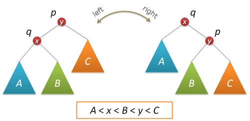
Application of a special insertion of a new key is the essential component of randomization. As a result of insertion, the new key is in the tree root. This information is useful in many ways, as the access to recently added keys is really fast, hello to self-organizing lists. To carry out the insertion in the root, we are going to need the rotate function that performs a local transformation of the tree.

Do not forget to update the size of subtrees and return a new tree root.
node* rotateright(node* p) // right rotation round p node
{
    node* q = p->left;
    if( !q ) return p;
    p->left = q->right;
    q->right = p;
    q->size = p->size;
    fixsize(p);
    return q;
}
node* rotateleft(node* q) // left rotation round q node
{
    node* p = q->right;
    if( !p ) return q;
    q->right = p->left;
    p->left = q;
    p->size = q->size;
    fixsize(q);
    return p;
}
Now, let’s perform the insertion in the root. First of all, insert recursively a new key in the root of the left or the right subtrees (depending on the result of comparing with the root key) and perform a right (left) rotation that raises the necessary node to the tree root.
node* insertroot(node* p, int k) // inserting a new node with k key in p tree
{
    if( !p ) return new node(k);
    if( k<p->key )
    {
        p->left = insertroot(p->left,k);
        return rotateright(p);
    }
    else
    {
        p->right = insertroot(p->right,k);
        return rotateleft(p);
    }
}

Randomized Insertion
We have finally made it to randomization. At the moment, we have two insertion functions – a simple one and the one in the root. Let’s make a randomized insertion from them. It is known that if we mix all the keys beforehand and build a tree from them (the keys are inserted according to a standard scheme in order that has been achieved after hashing), the built tree will be quite balanced (its height will be around 2log2n compared to log2n for a perfectly balanced tree). Please note, that in this case any of source keys can be a root. But what should we do, if we do not know beforehand, what keys we will have (for instance, they’re introduced into system during a tree usage). But all of that is actually simple. Since any key (including the one we will insert in the tree now) can be a root with 1/(n+1) probability (n is the tree size before insertion), we execute the insertion with the given probability and a recursive insertion in the right or the left subtree (depending on the key value in the root) with 1-1/(n+1) probability.
node* insert(node* p, int k) // a randomized insertion of a new node with k key in p tree
{
    if( !p ) return new node(k);
    if( rand()%(p->size+1)==0 )
        return insertroot(p,k);
    if( p->key>k )
        p->left = insert(p->left,k);
    else
        p->right = insert(p->right,k);
    fixsize(p);
    return p;
}


Key Deletion

So, we have an imbalanced (at least in some way) tree. As for now, it does not support key deletion. That’s exactly what we are going to solve now. The described in manuals variant operates fast, but does not really look nice (in contrast to insertion). We will follow a different path. Before deleting nodes, we will learn how to join trees together. Let there be given two trees with p and q roots. Any key of the first tree is less than any key of the second tree. It is required to join these two trees into a single one. We can accept any of two roots as the root of a new tree, let it be p. In this case, we can leave the left p subtree as it is and fix the join of two trees to p on the right – the right p subtree and the whole q tree (they meet all the requirements).


On the other hand, we can just as well make q node the root of a new tree. In the randomized implementation, we choose between these two alternatives in a random manner. Assume that the size of the left tree is n, while the right tree size is m. Then p is chosen to be a new root with n/(n+m) and q is chosen with m/(n+m) probability.
node* join(node* p, node* q) // joining two trees
{
    if( !p ) return q;
    if( !q ) return p;
    if( rand()%(p->size+q->size) < p->size )
    {
        p->right = join(p->right,q);
        fixsize(p);
        return p;
    }
    else
    {
        q->left = join(p,q->left);
        fixsize(q);
        return q;
    }
}


Now everything is ready for deletion. We are going to delete by the key. Look for the node with the specified key (reminding you that all keys are different) and delete this node from the tree. The search stage is the same as searching. Then we join the right and the left subtrees of the found node, delete the node and return the root of the joined tree.
node* remove(node* p, int k) // deleting from p tree the first found node with k key
{
    if( !p ) return p;
    if( p->key==k )
    {
        node* q = join(p->left,p->right);
        delete p;
        return q;
    }
    else if( k<p->key )
        p->left = remove(p->left,k);
    else
        p->right = remove(p->right,k);
    return p;
}
Implementation simplicity and beauty are the doubtless advantages of Binary Search Trees. But what’s the drawback? What do we pay for it? First of all, the additional memory for storing subtrees sizes. One integer-valued field per each node. As for Red-Black Trees, we can do without additional fields. On the other hand, the tree size information is not useless, since it allows to organize the access to the data by number (sampling or order statistics search), which transforms our tree into an ordered array with feasible insertion and deletion of any elements. Secondly, though the operation time is logarithmic, the proportionality coefficient will not be small as all the operations are performed in two passes (up and down). Besides, insertion and deletion require random numbers. But there’s also the good news. At the search stage everything should operate really fast. Finally, logarithmic time is not guaranteed. There’s always a chance that a tree will be ill-balanced. But when there are ten thousand of nodes, such possibility is so negligible that it’s worth risking.